
What Is a Language Model?
The Function Hiding Behind Every API Call

Five sentences to take with you
A modern language model is a function: text in, text out, with hundreds of billions of frozen numbers between them.
Tokens become vectors, the vectors flow up a stack of identical layers, the last vector becomes a probability over the next word, sampling picks one, and the loop repeats.
A 10-word prompt becomes ~53,000 floats before the model touches it; a 2,000-word answer is 2,500 sequential forward passes through the entire stack.
Every named technique in the news (MoE, FlashAttention, RoPE) is a swap for one specific component of that pipeline; the shape itself has barely changed since 2017.
The model has no memory between calls, which is why the entire agent industry exists.
You can fit a frontier model on the back of a napkin.
That sounds wrong because the press treats GPT-class systems as inscrutable. They aren’t. Strip away the marketing and what’s left is a function. You give it text. It gives you text. In between, hundreds of billions of frozen numbers process your input through a fixed sequence of operations and produce one new word, one at a time, until the response stops.
Once you see this picture, the rest stops feeling magical. You can read the DeepSeek V3 paper, or the Llama technical report, or whatever drops next month, and know exactly which component each new trick is replacing. That’s the goal of this piece.
The whole picture in one paragraph
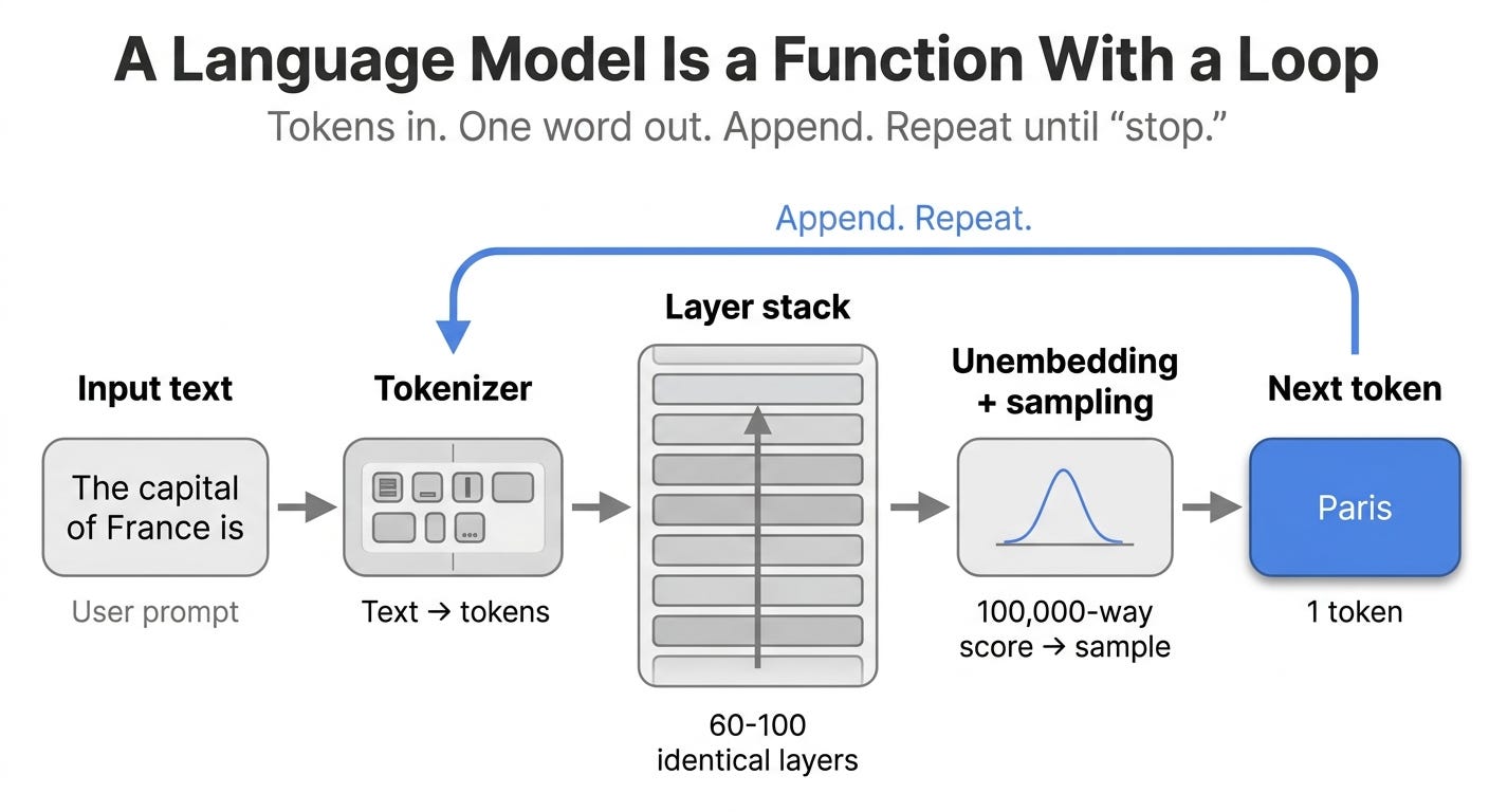
A language model is a stack of identical layers. Tokens enter as vectors. The vectors flow up the stack picking up context as they go. At the top, the last vector gets projected back to a vocabulary score that determines the next word. Sampling picks one. The picked word is appended to the input. The whole stack runs again. This continues until the model emits a special “stop” token or hits a length limit.
That’s it. That’s an LLM. Everything else in any paper, diagram, or benchmark is detail underneath those sentences. The rest of this article unpacks each phase.
What goes in: text becomes a slab of numbers
Text gets converted to numbers before the model sees it. Your prompt is broken into tokens, small chunks roughly the size of a syllable or short word, and each token is replaced with a fixed-length vector of numbers that represents what the token means to the model.
If a model has a 100,000-token vocabulary and 4,096-dimensional vectors, its vocabulary is a giant table holding 100,000 by 4,096 numbers. Each row is one token’s vector. When you send a prompt, your sentence gets converted into a stack of those rows.
A 10-word input becomes roughly 13 rows by 4,096 columns. That’s about 53,000 floating-point numbers. By the time the model touches your prompt, it doesn’t look like text. It looks like a small slab of floats.
Two details matter later. The table of token-to-vector mappings is called the embedding table, and it’s the model’s first set of learned parameters. A 100,000 by 4,096 table holds 410 million parameters by itself. The conversion from text to tokens is done by a separate piece of code called the tokenizer, a frozen lookup that doesn’t learn during training.
Different labs make different choices. GPT-2 used 50,257 tokens. Llama 1 used 32,000. Llama 3 jumped to 128,000. Qwen 2.5 uses 152,064. Bigger vocabularies mean fewer tokens per sentence (cheaper inference) but more parameters in the embedding table. Most 2026 labs converge between 100,000 and 200,000.
What happens inside: a stack of identical layers
The slab of vectors flows through a tower of identical layers. A modern model has between 32 and 128 of them. Llama 3.1 70B has 80. DeepSeek V3 has 61. Mistral Large has 88. Layers are stacked one after another. The output of layer 1 is the input to layer 2, the output of layer 2 is the input to layer 3, and so on, all the way to the top.
Every layer does two things. Always two. Never more.
The first thing a layer does is mix information across positions. This is the attention operation. Each token gets to look at every other token in the sentence and pull in a weighted blend of their vectors. After attention, a token’s vector contains not just its own meaning but a smear of relevant context. What came before. What’s nearby. What matters for understanding.
The second thing a layer does is mix information within each position. This is the feed-forward operation. Each token’s vector, now containing context, gets pushed through a small neural network that operates on it independently of the other tokens. This step is where most of the model’s factual knowledge lives. Geva et al. (2021) showed empirically that ablating individual feed-forward neurons removes specific facts from a model’s recall. The fact that Paris is the capital of France lives somewhere in there, in specific neurons, on a specific layer.
[Diagram: one layer, attention then feed-forward, both wrapped in residual connections]
Both operations sit on a residual stream, which means the input to each operation is added back to its output. The residual stream is what lets a stack of 80 layers refine a vector progressively without losing track of what was originally there. He et al. (2015) introduced residual connections in image recognition. Vaswani et al. (2017) carried them into the transformer. Without them, training a stack this deep would not converge.
That’s a layer. Stack 80 of them. Glue an embedding table on the front. Glue an unembedding projection on the back. You have a frontier model.
What comes out: one word at a time
When the stack of vectors emerges from the top layer, the model has to turn them back into text. It does this by taking the last token’s vector, the one in the position that just got attended to by everything before it, and projecting it back against the vocabulary table from the start. The result is a list of 100,000 scores, one per possible next token. Higher scores mean “more likely.”
A function called softmax turns those scores into probabilities that sum to 1. Then a sampling strategy picks one. The highest one (greedy), or one drawn weighted by the probabilities (temperature sampling), or one of the top k, or one of the top p by cumulative probability. Holtzman et al. (2019) introduced top-p, also called nucleus sampling, and it’s now the default in most APIs.
The picked token is appended to the input. The whole stack runs again. Another token is picked. And another. Until the model emits a special “stop” token or hits a length limit.
That’s where the response comes from. One token at a time. A full sentence is the result of running the model dozens or hundreds of times in sequence. Reasoning models that “think before they answer” do this for thousands of tokens before they show you anything.
Why your API calls are slow AND expensive at the same time
Every token of output costs one forward pass through the entire stack. A 200-word answer is roughly 250 forward passes. A 2,000-word answer is 2,500. A reasoning trace can hit 50,000. The model doesn’t know in advance how long it’ll take. It just keeps generating until it decides to stop.
That generation is fundamentally sequential. The next token depends on the previous one, which depends on the one before. You can’t parallelize “what’s the next word.” This is why streaming exists: the model emits tokens as it generates them so the user perceives motion, even though the total time hasn’t changed.
It’s also why inference costs more than people expect. Every active user, every minute, is running the entire stack repeatedly. Sardana and Frankle (2023) estimated that for a popular model, inference compute exceeds training compute within a few weeks of launch. We’ll come back to that on Saturday.
Where the parameters actually live
“70 billion parameters” sounds abstract. Here’s where the numbers actually sit.
Llama 3.1 70B has 70 billion parameters. Most live inside the 80 feed-forward networks (one per layer). A smaller share is in the attention components, which take more time to run but use fewer parameters. Some are in the embedding table at the entrance and the unembedding projection at the exit.
DeepSeek V3 has 671 billion total parameters. Only 37 billion fire for any given token, because V3 is a Mixture of Experts model: most tokens activate roughly 9 of its 256 experts plus 1 always-on shared expert. So while V3 holds nine times more knowledge than Llama 70B, it runs at roughly half the active-parameter cost.
Useful rule of thumb: count active parameters to know the cost of running the model, count total parameters to know how much it has learned. The two can differ by 20x in MoE models. Press headlines quote totals because they’re bigger. The serving stack cares about actives.
A common misconception, and the correction
Most people think a language model “looks up” answers the way a search engine returns a result. It doesn’t. It computes them.
When you ask GPT or Claude what the capital of France is, the model doesn’t search a database for “France: capital.” It runs your tokenized prompt through 60 to 100 layers of matrix multiplication. “Paris” emerges because gradient descent settled the parameters such that, given a sentence ending in “the capital of France is,” the highest-probability next token is “Paris.”
There is no lookup. No fact is stored as text. The “fact” is a particular pattern of activations across particular layers, learned from seeing the assertion many times during training. Geva 2021’s finding (ablating feed-forward neurons removes facts) is what you’d expect of a system that computes facts from learned weights, not one that stores them.
This matters practically: every behavior you observe in an LLM is the output of the same matrix multiplication. Reasoning. Refusal. Hallucination. Code generation. Tone. All computed by the same machinery. Treating any of them as “different modes” is misleading. There’s only one mode.
What works today, what doesn’t
What works: the picture above. Decoder-only transformers, scaled between roughly 7 billion parameters (small open models) and 1.6 trillion total parameters (frontier MoE), trained on tens of trillions of tokens, post-trained for instruction following and reasoning, served behind aggressive inference engineering. Every frontier API is this, underneath.
What doesn’t yet work: anything that asks the model to reliably hold information that wasn’t in training and isn’t in the current context. The model has no memory between calls. Each call starts cold. Whatever you want it to remember, you feed it in the prompt, every time. The entire agent industry exists in large part to manage this constraint.
What also doesn’t work: assuming bigger is always better. Hoffmann et al. (2022) showed that for a fixed compute budget, smaller models trained on more tokens beat bigger models trained on fewer. Press headlines still lead with parameter counts. The actual frontier has shifted to “right-sized” models trained for longer.
Hold this picture and the rest of the field becomes navigable. Tomorrow, we zoom in on the most-revised, most-named part of the engine: the attention half of every layer, and why “every layer does exactly two things” is a stronger statement than it sounds.
References and Further Reading
Vaswani et al., Attention Is All You Need (2017). The transformer architecture in six pages. Still the cleanest introduction.
He et al., Deep Residual Learning for Image Recognition (2015). Where residual connections come from. Without these, training deep stacks doesn’t converge.
Geva et al., Transformer Feed-Forward Layers Are Key-Value Memories (2021). Empirical evidence that the feed-forward sublayer is where the model stores facts.
Holtzman et al., The Curious Case of Neural Text Degeneration (2019). Why we need top-p sampling instead of greedy decoding.
Hoffmann et al., Training Compute-Optimal Large Language Models (2022). The Chinchilla scaling laws. Why bigger isn’t always better.
Sardana and Frankle, Beyond Chinchilla-Optimal: Accounting for Inference in Language Model Scaling Laws (2023). The reason most labs train on more tokens than Chinchilla recommends, and why inference cost dominates within weeks of launch.
Karpathy, Let’s build GPT: from scratch, in code, spelled out (2023). Two hours of seeing a transformer assembled line by line. The single best companion video for this article.
3Blue1Brown, But what is a GPT? Visual intro to transformers (2024). A different teaching style. Also excellent.
Phuong and Hutter, Formal Algorithms for Transformers (2022). The mathematician’s version of this article.