
Every Transformer Layer Does Exactly Two Things. Always Two. Never More.

Five sentences to take with you
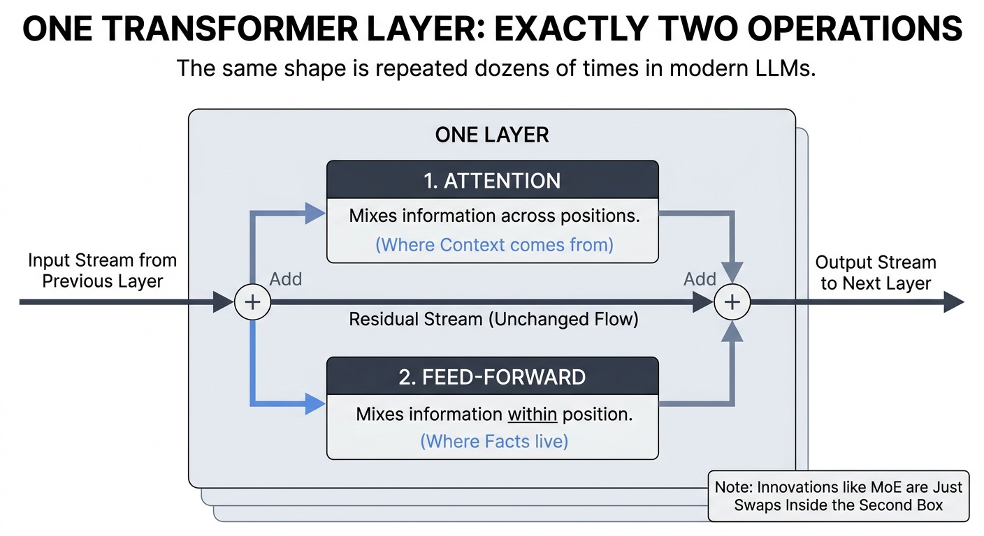
Every layer in every modern LLM does the same two operations in the same order: mix across positions (attention), then mix within each position (feed-forward).
Attention is where context comes from; feed-forward is where facts live, and Geva et al. (2021) showed you can ablate specific neurons to remove specific facts.
The residual stream, borrowed from 2015 image-recognition research, is the unsung hero; without it, an 80-layer stack would never train.
Almost every architecture innovation since 2017 (MoE, MLA, GQA, RoPE, SwiGLU) is a swap inside one of those two boxes, and the boxes themselves haven’t moved.
Once you hold this picture, every “revolutionary” architecture paper becomes a labeled callout against the same eight-year-old shape.
Modern frontier model architecture diagrams look terrifying.
You’ve probably seen one. A page-tall cathedral of boxes labeled with acronyms: GQA, RoPE, RMSNorm, SwiGLU, MLA, MoE Router, MTP heads, decoupled this, sparse that. The implication is that each new model is a fundamentally new kind of system.
It isn’t. The cathedral is the same cathedral it was in 2017. What changes is which stones get swapped for cheaper or smarter versions.
The simplest way to see this is to look at one layer. Just one. Once you can hold a single layer in your head, the entire field becomes a series of footnotes against that picture.
Two operations. That’s the whole thing.
A transformer layer does exactly two things, in this order:
Mix information across positions. This is the attention sublayer. Each token in the sequence gets to look at every other token and pull in a weighted blend of their vectors.
Mix information within each position. This is the feed-forward sublayer. Each token’s vector, now containing context, gets pushed independently through a small neural network.
Both operations sit on a residual stream. The input to each sublayer is added back to its output before moving on. Both are preceded by a normalization step. That’s the layer.
Stack 80 of these and you have Llama 3.1 70B. Stack 61 and you have DeepSeek V3. Stack 88 and you have Mistral Large. The numbers vary. The shape doesn’t.
[Diagram: one layer, input, norm, attention, residual add, norm, feed-forward, residual add, output]
If you remember nothing else from this series, remember those two operations and the residual stream connecting them. Everything else is variations on a theme.
Attention: where context comes from
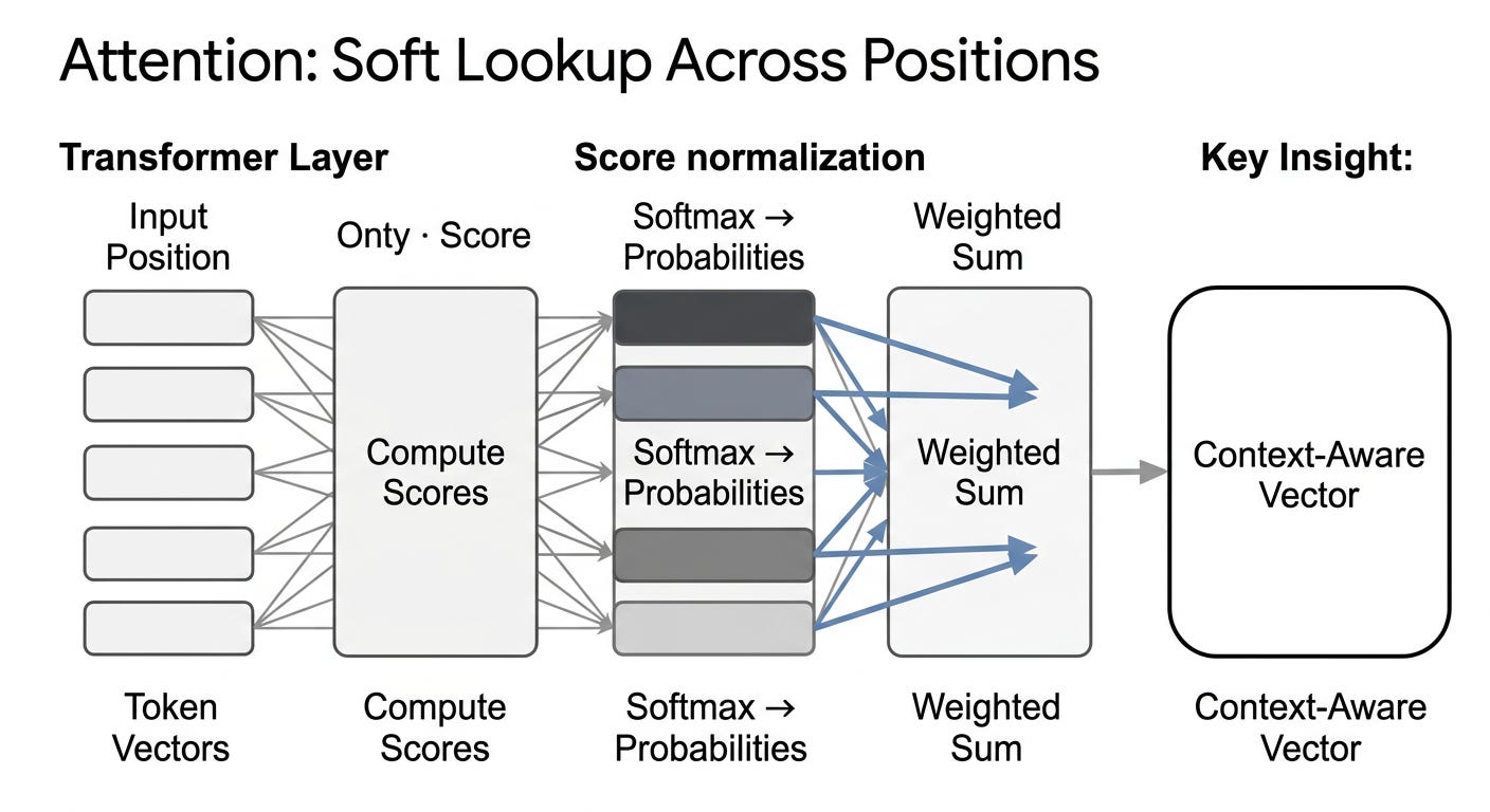
When a token’s vector arrives at the attention sublayer, it carries only what that token “means” by itself. After attention, it carries a smear of everything around it that’s relevant.
The mechanism is a weighted average. Each token computes a score against every other token in the context. Higher scores mean “this other token matters more for understanding me.” A softmax turns the scores into a probability distribution. The token’s new vector is the probability-weighted sum of the values held by every position it attended to.
That’s it. That’s attention. It’s a soft, learned lookup over the rest of the sequence.
The reason this single operation is so powerful: it’s the only place in the model where information can flow between positions. Take attention out and each position is processed independently from end to end, never seeing what its neighbors said. The model wouldn’t be able to handle pronouns. It wouldn’t track topic. It would have no syntax.
When you read about attention variants in 2026 (Multi-Head Attention, Grouped-Query Attention, Multi-Head Latent Attention, sliding window attention, sparse attention, FlashAttention), every one of them is solving an engineering problem with this same mechanism: how to make the score-and-weighted-sum part faster, smaller, or more parallel. The mathematical operation is unchanged.
Feed-forward: where facts live
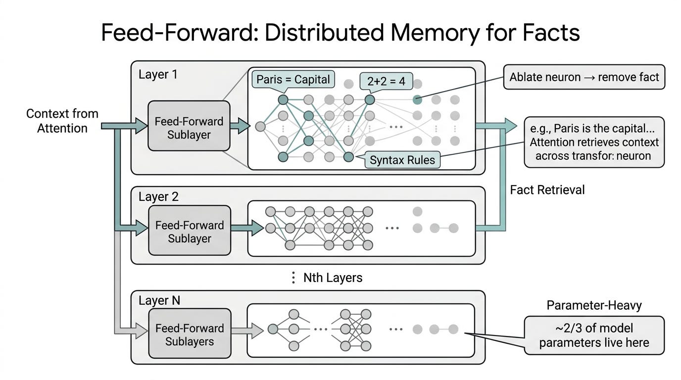
After attention, each token’s vector is independently pushed through a feed-forward network. Two linear projections with a non-linearity in between. Same network applied identically to every position.
This part doesn’t sound exciting. It is.
Geva et al. (2021) showed empirically that ablating individual neurons in the feed-forward sublayer removes specific facts from the model’s recall. The fact that Paris is the capital of France lives somewhere in there, on a specific layer, in specific neurons. You can find it. You can break it. The word “memory” in their paper title is literal.
That changes how you should think about what the feed-forward layer is. It’s not a generic processing step. It’s distributed key-value storage, scattered across all 80 (or 61, or 88) layers, that the attention mechanism reads from to produce its output.
A useful way to picture it: attention says “given this context, what should I retrieve?”, and feed-forward is the warehouse that holds the retrievable items. The two sublayers complement each other. One contextualizes; the other recalls.
This is also why the feed-forward sublayer holds most of the parameters. In Llama 3.1 70B, the FFN is roughly two-thirds of the total parameter count. Most of what the model “knows” is stored there.
The residual stream: the part nobody talks about
Both sublayers are wrapped in a residual connection. The input to the operation is added back to its output. Sounds trivial. Isn’t.
Without residual connections, training a stack of 80 transformer layers does not converge. Period. The gradients vanish. The early layers stop learning. The model stays at random performance no matter how long you train.
He et al. (2015) introduced residual connections in image recognition. They were trying to train networks deeper than 20 layers, which kept getting worse the deeper they went. The fix was a connection from each layer’s input to its output, letting gradients flow backward through the addition. Vaswani et al. (2017) carried the trick into the transformer.
The picture in your head should be: a “stream” of vectors flowing up from the embedding table through 80 layers to the output. Each sublayer doesn’t replace the stream’s contents. It adds a refinement. Position 1’s vector at layer 5 is the same vector it was at layer 4, plus a small modification from attention, plus another small modification from feed-forward.
That’s why deep transformers can keep learning. Each layer makes a small, additive contribution. The model can decide, layer by layer, how much to refine and how much to leave alone.
If a single architectural choice deserves credit for the modern era of language models, it’s the residual stream. Every other refinement (better attention, better activations, better positional encoding) sits on top of it.
The one big variant: Mixture of Experts
If “every layer does exactly two things” is the rule, MoE is the one true exception. Or rather: MoE is the most aggressive swap inside the second box.
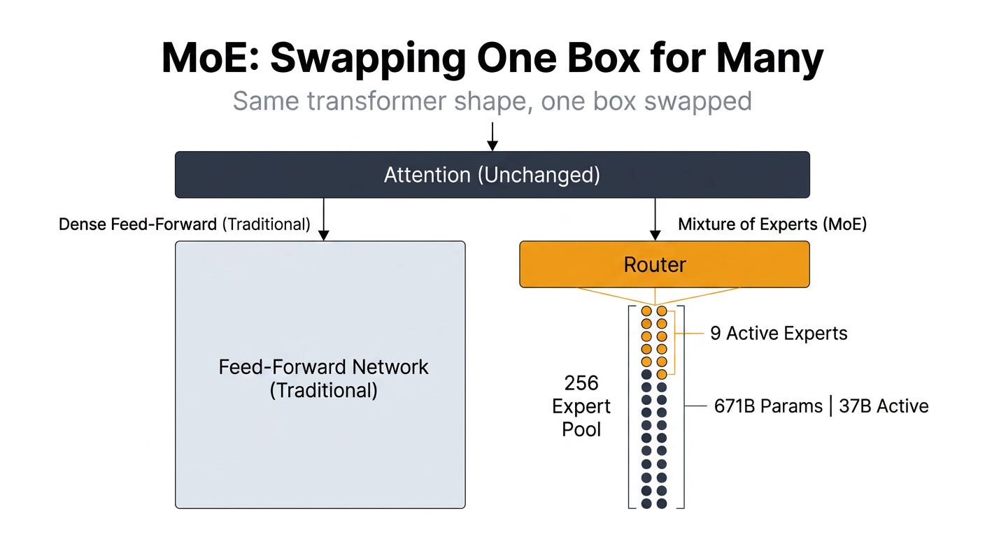
In a Mixture of Experts model, the feed-forward sublayer isn’t one network. It’s a router plus a pool of expert networks. When a token arrives, the router picks a small number (usually 2 to 9) of experts from the pool. The token is processed by those experts, and only those experts, before continuing.
DeepSeek V3 has 256 routed experts plus 1 always-on shared expert per layer, with roughly 9 active per token. Total parameter count: 671 billion. Active parameters per token: 37 billion. The model holds nine times more knowledge than Llama 70B but runs at roughly half the active-parameter cost.
This sounds revolutionary. It isn’t. The router replaces one feed-forward network with many. The attention sublayer is unchanged. The residual stream is unchanged. The number of layers is in the same range (61, vs Llama’s 80). The shape is the same. One box got swapped.
Liu et al. (2024), the DeepSeek V3 technical report, is worth reading specifically because it shows how many named subsystems a single frontier MoE model carries (Multi-Head Latent Attention, decoupled-RoPE, Multi-Token Prediction, expert routing tricks). Each one is a swap into the same two-box picture. None of them changes the picture.
Why the shape hasn’t moved in 8 years
Compare the structure of Llama 3.1 70B (2024) to GPT-2 (2019) to the original transformer paper (2017). Same idea. Decoder-only stack, identical layers, attention then feed-forward, residual stream, normalization in between. The numbers are different. The shape isn’t.
What did change in eight years:
Position encoding. Sinusoidal in 2017 → learned in GPT-2 → RoPE almost everywhere now. Tells attention which token came first.
Activation function in the feed-forward. ReLU → GeLU → SwiGLU. Small efficiency wins.
Normalization. LayerNorm → RMSNorm in most modern models. Same idea, less computation.
Attention efficiency. Multi-Head → Multi-Query → Grouped-Query → Multi-Head Latent. Each variant makes the KV cache smaller without changing what attention does mathematically.
MoE in the second box. Replaces one feed-forward network with many specialized ones.
Each is a real engineering improvement. None changes the architecture. The cathedral is still the cathedral. We swapped some stones.
This matters because every time the press calls a new model “revolutionary,” the actual change is almost always a swap into one of the two boxes. Knowing the shape lets you read past the marketing and ask the only question that matters: which box did they touch, and how much cheaper or smarter is the new version?
What this picture buys you
Three things, concretely.
You can read any new architecture paper. The introduction will spend pages explaining why the new technique matters. You can skip most of it. Find the diagram. Locate the two boxes. See which one was swapped. Read the rest of the paper through that lens.
You can debug your intuitions. “Why does the model know facts but get reasoning wrong?” Because facts live in feed-forward and reasoning emerges from attention chaining context across many layers. Different sublayers; different failure modes.
You can reason about cost. Attention is parameter-light but compute-heavy (especially as context grows). Feed-forward is parameter-heavy but compute-flat per token. When you see a model with 671 billion parameters running at the cost of a 37-billion-parameter dense model, you know the difference is in the feed-forward box, because that’s where MoE lives.
Tomorrow we follow the layer’s output to its actual destination: the data center. We’ll see why training a 70-billion-parameter model costs $50 million but inference costs more within weeks of launch.
References and Further Reading
Vaswani et al., Attention Is All You Need (2017). The transformer architecture in six pages. The shape it introduced is the shape we still use.
He et al., Deep Residual Learning for Image Recognition (2015). Residual connections, originally for image classification. Without them, 80-layer stacks don’t train.
Geva et al., Transformer Feed-Forward Layers Are Key-Value Memories (2021). Empirical evidence that the feed-forward sublayer literally stores facts.
Liu et al., DeepSeek-V3 Technical Report (2024). A modern MoE frontier model with every named subsystem turned on. Useful precisely because it shows how all the swaps stack into the same shape.
Dubey et al., The Llama 3 Herd of Models (2024). The dense-architecture counterpart. Same shape, different choices in each box.
Phuong and Hutter, Formal Algorithms for Transformers (2022). The mathematician’s version of this article.
Karpathy, Let’s build GPT: from scratch, in code, spelled out (2023). Two hours of building a transformer line by line. The fastest way to internalize the two-box picture.